Tutorial of pydefect
This page explains how to use the pydefect code.
Note 1: Pydefect currently supports only the Vienna Ab-initio Simulation Package (VASP). Therefore, it assumes the use of VASP-specific input and output file names (e.g., POSCAR, POTCAR, OUTCAR) as well as computational methods such as periodic boundary conditions.
Note 2: The units used in Pydefect follow the VASP convention: energy is in electronvolts (eV) and length is in angstroms (Å).
Note 3: At present, only nonmagnetic host materials are supported.
The workflow for point-defect calculations in non-metallic solids is illustrated below. Some tasks can be performed in parallel, while others must be carried out sequentially. Since these procedures are often complex and time-consuming, researchers are prone to making mistakes.
The primary goal of pydefect is to provide an automated system
for point-defect calculations in non-metallic materials.
This helps researchers save time and minimize human error.
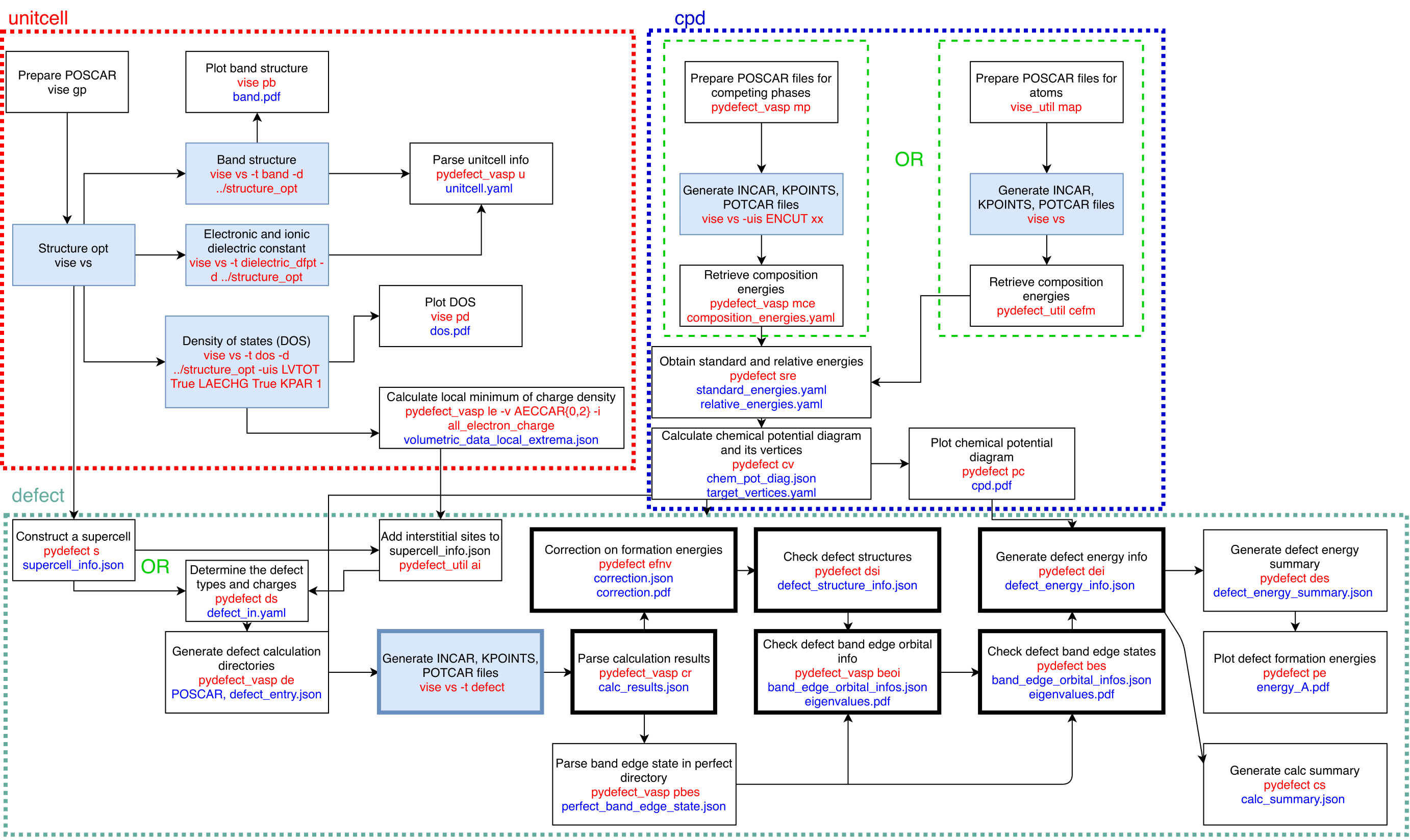
This cheat sheet is divided into three parts: unitcell, chemical potential diagram (cpd), and defect, each corresponding to a working directory, as illustrated below.
Red text indicates related commands, while blue text denotes the files generated by those commands. Branches represent alternative workflows or options. Filled blue rectangles indicate steps that require VASP calculations. Bolded rectangles represent steps that involve multiple directories related to the considered defects. Green rectangles indicate optional steps.
Here, we assume the following directory structure.
The placeholder <project_name> typically represents the name of the target material,
optionally including its crystal structure — for example, rutile-TiO:sub:2``.
<project_name>
 │
 ├ pydefect.yaml
 ├ vise.yaml
 │
 ├ unitcell/ ── structure_opt/
 │            ├ band/
 │            ├ dielectric/
 │            └ dos/
 │
 ├ cpd/ ──── <competing_phase 1>
 │       ├── <competing_phase 2>
 │           ....
 │
 └ defect/ ── perfect/
            ├─ Va_X_0/
            ├─ Va_X_1/
            ├─ Va_X_2/
             ...
We recommend that users follow the same directory structure if possible. The details of the workflow are explained step by step, using an example of MgAl₂O₄ calculated with the PBEsol functional.
In :code:pydefect, there are five main command-line tools:
pydefect
pydefect_vasp
pydefect_util
pydefect_vasp_util
pydefect_print
The commands pydefect_vasp and pydefect_vasp_util are related to VASP,
while pydefect and pydefect_util are independent of any specific DFT code.
Commands with the suffix _util are not strictly necessary, but they can be useful in certain situations.
Each subcommand supports a variety of arguments.
You can always display the help message using the -h flag. For example:
pydefect s -h
to view detailed information.
1. Relaxation of the unit cell
Point-defect calculations are typically performed on a theoretically relaxed structure, using a specified exchange-correlation functional and projector augmented wave (PAW) potentials. This ensures that the structure is free from artificial strain and stress, which can otherwise introduce unwanted dependencies on the supercell size. Therefore, the first step is usually to optimize the lattice constants and the fractional atomic coordinates in the unit cell.
We first prepare the POSCAR file of the pristine bulk unit cell,
and create the unitcell/ directory and its subdirectory unitcell/structure_opt/
(using mkdir -p unitcell/structure_opt/), then move into it.
(In this tutorial, any name ending with / indicates a directory.)
When pydefect needs to generate VASP input files,
namely INCAR, POTCAR, and KPOINTS,
we use the vise
(short for vasp integrated supporting environment),
which creates input files for various tasks and exchange-correlation (XC) functionals.
vise depends on pymatgen, and therefore,
as explained in pymatgen usage page 1 or
page 2,
you need to set the PMG_DEFAULT_FUNCTIONAL and PMG_VASP_PSP_DIR
in the .pmgrc.yaml file located in your home directory. For example:
PMG_DEFAULT_FUNCTIONAL: PBE_54
PMG_MAPI_KEY: xxxxxxxxxxxxxxxx
PMG_VASP_PSP_DIR: /home/kumagai/potcars/
In pydefect, PMG_MAPI_KEY is required to query
POSCAR files and the total energies of competing materials.
Input files for optimizing a unit cell using the PBEsol functional can be generated with the following command:
vise vasp_set -x pbesol
Here, vasp_set, or its abbreviation vs,
is a subcommand of the main vise function.
Similarly, all subcommands in pydefect and vise have their own abbreviations.
Since the PBE functional is the default in vise,
we use the -x argument to switch the XC functional to PBEsol.
Note that structure optimization generally needs to be repeated with a 1.3× larger cutoff energy until both the forces and stresses are well converged at the first ionic step. See the vasp manual for further details.
This iterative process is not supported by pydefect,
but it can easily be implemented using a simple shell script.
In pydefect, users can control various default parameters
via the vise.yaml file used by vise.
See the vise documentation for more information.
The set of configurable parameters can be found in defaults.py in pydefect.
2. Calculation of band, DOS, and dielectric tensor
We then calculate the band structure (BS), density of states (DOS), and dielectric constants. In defect calculations, the BS is used to determine the valence band maximum (VBM) and conduction band minimum (CBM), while the dielectric constant, defined as the sum of the electronic (ion-clamped) and ionic dielectric tensors, is required for correcting the defect formation energies.
First, create the band/, dos/, and dielectric/ directories inside unitcell/,
copy the POSCAR file from unitcell/structure_opt/,
and run the following command in each directory:
vise vs -x pbesol -t band -pd ../structure_opt
vise vs -x pbesol -t dos -pd ../structure_opt -uis LVTOT True LAECHG True KPAR 1
vise vs -x pbesol -t dielectric_dfpt -pd ../structure_opt
The additional user_incar_settings (abbreviated as uis) in the dos directory
are used to generate volumetric data for the electrostatic potential and all-electron charge density.
vise also provides plotting utilities for both the band structure (BS) and density of states (DOS).
See the vise documentation for details.
3. Gathering unit cell information for point-defect calculations
We next collect the bulk information,
namely the band edges and electronic and ionic dielectric tensors
using the unitcell (= u) sub-command.
pydefect_vasp u -vb band/vasprun-finish.xml -ob band/OUTCAR-finish -odc dielectric/OUTCAR-finish -odi dielectric/OUTCAR-finish -n MgAl2O4
Here, the electronic and ionic dielectric constants can be set
with different OUTCAR files.
Then, unitcell.yaml is generated, which will be used for analyzing defect calculations later.
system: MgAl2O4
vbm: 4.0183
cbm: 9.2376
ele_dielectric_const:
- - 3.075988
  - 0.0
  - -0.0
- - 0.0
  - 3.075988
  - 0.0
- - -0.0
  - -0.0
  - 3.075988
ion_dielectric_const:
- - 5.042937
  - -0.0
  - -0.0
- - -0.0
  - 5.042937
  - 0.0
- - -0.0
  - 0.0
  - 5.042937
Of course, the users can also create it by hand.
4. Calculation of competing phases
When a defect is introduced, atoms are exchanged with hypothetical atomic reservoirs within a thermodynamic framework. To calculate the free energy of defect formation, often approximated by the defect formation energy, we need to determine the chemical potentials of the atoms involved in the defect. Typically, these chemical potentials are chosen under the condition where the host material coexists with its competing phases, as determined from a chemical potential diagram (CPD).
To set up this process, we create directories under cpd/.
We retrieve POSCAR files of stable or slightly unstable competing phases
from the Materials Project database (MPD).
This requires an MP API key, as described earlier.
For example, to obtain competing phases for MgAl2O4 with energies above the convex hull less than 0.5 meV/atom, use:
pydefect_vasp mp -e Mg Al O --e_above_hull 0.0005
This command generates directories like:
Al2O3_mp-1143/  Al_mp-134/  Mg149Al_mp-1185596/  Mg17Al12_mp-2151/
MgAl2O4_mp-3536/  MgAl2_mp-1094116/  MgO_mp-1265/  Mg_mp-1056702/  mol_O2/
To reduce computational time in this tutorial, we remove Mg149Al_mp-1185596/.
Each directory contains a POSCAR file and a prior_info.yaml file.
The prior_info.yaml file includes information retrieved from the MPD
that is useful for setting VASP calculation conditions via vise.
For example, Mg_mp-1056702/prior_info.yaml contains:
band_gap: 0.0
data_source: mp-1056702
total_magnetization: 0.0007357
indicating that Mg is a non-magnetic metal.
vise uses this file to determine the k-point density in KPOINTS
and whether spin polarization is needed via the ISPIN tag in INCAR.
If any value is clearly incorrect, the user can modify it manually.
The molecules O2, H2, N2, NH3, and NO2
are not retrieved from MPD but are instead generated by pydefect,
since MPD often treats them as solids, which is unsuitable for defect calculations.
We then generate the INCAR, POTCAR, and KPOINTS files for these systems.
A common cutoff energy, ENCUT, is required for comparing total energies.
This value is set to 1.3 times the maximum ENMAX among the constituent POTCARs.
For example, in the case of MgAl₂O₄, the ENMAX values for Mg, Al, and O are 200.0, 240.3, and 400.0 eV, respectively.
Therefore, we set ENCUT = 520.0 using vise:
for i in *_*/; do cd $i; vise vs -uis ENCUT 520.0 -x pbesol; cd ../; done
The target material (MgAl₂O₄ in this case) has already been calculated under the same condition, so we do not need to repeat the calculation. Instead, create a symbolic link with:
ln -s ../unitcell/structure_opt MgAl2O4_unitcell
and remove the MgAl2O4_mp-3536/ directory.
However, if a different ENMAX is used to match dopant atoms with larger values,
you need to recalculate it to maintain consistency.
Note
If any of the competing phases is a gas,
set ISIF = 2 to avoid relaxing the lattice constants
(see VASP manual),
and use Gamma-point-only sampling in KPOINTS.
These settings are automatically adjusted by vise via prior_info.yaml.
After completing the VASP calculations, you can generate the composition_energies.yaml file,
which collects the total energies per formula unit using the make_composition_energies (mce) sub-command:
pydefect_vasp mce -d *_*/
If you rename vasprun.xml and OUTCAR files during calculations
(e.g., to vasprun-finish.xml and OUTCAR-finish),
specify the new names in vise.yaml as follows:
# VASP file names
outcar: OUTCAR-finish
vasprun: vasprun-finish.xml
See Tutorial for vise.yaml for details.
Next, create relative_energies.yaml and standard_energies.yaml
using the standard_and_relative_energies (sre) sub-command:
pydefect sre
The standard_energies.yaml contains absolute energies under standard states:
Al: -4.08372115
Mg: -1.70955951
O:  -5.13918369
The relative_energies.yaml contains energies relative to the standard states:
Al2O3:     -3.14944023
Mg17Al12:  -0.02717980
MgAl2:     -0.01511851
MgAl2O4:   -3.09773128
MgO:       -2.83181863
To construct the CPD (convex hull), use the cpd_and_vertices sub-command:
pydefect cv -t MgAl2O4
To visualize the diagram, use the plot_cpd (pc) sub-command:
pydefect pc
This generates a file cpd.pdf. Binary and ternary CPDs appear as:
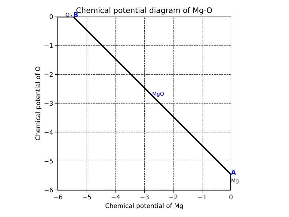
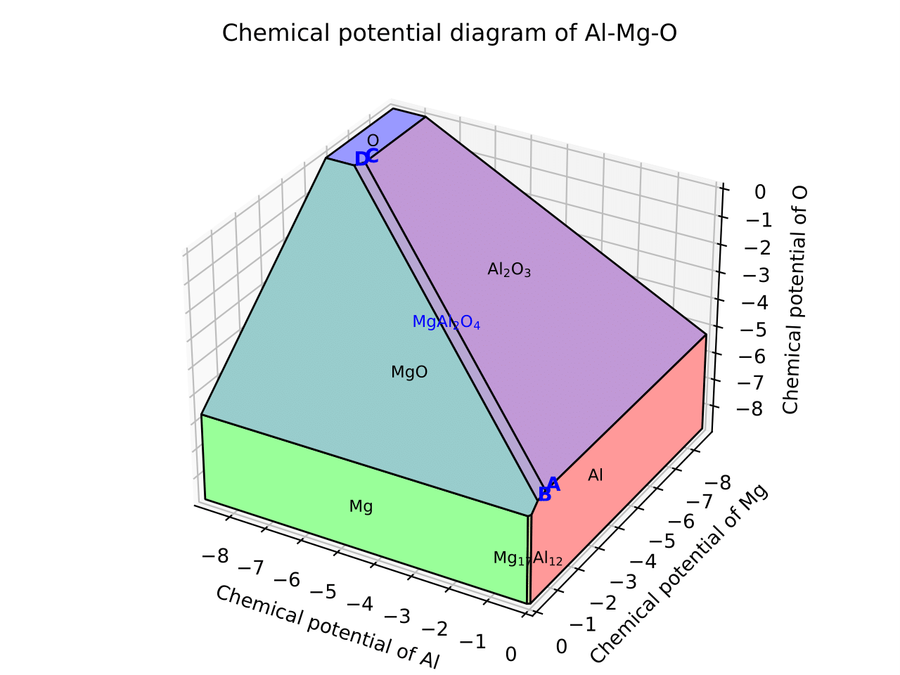
The vertices around the target compound are also shown:
target: MgAl2O4
A:
  chem_pot:
    Al: 0.0
    Mg: -0.68785
    O:  -5.24907
  competing_phases:
    - Al2O3
    - Al
  impurity_phases: []
B:
  chem_pot:
    Al: 0.0
    Mg: -0.32348
    O:  -5.34016
  competing_phases:
    - MgO
    - Al
  impurity_phases: []
C:
  chem_pot:
    Al: -7.87360
    Mg: -5.93692
    O:  0.0
  competing_phases:
    - Al2O3
    - O
  impurity_phases: []
D:
  chem_pot:
    Al: -8.01024
    Mg: -5.66364
    O:  0.0
  competing_phases:
    - MgO
    - O
  impurity_phases: []
To manually adjust the CPD energies, you can directly edit the relative_energies.yaml file.
Calculations of competing phases can be time-consuming.
If you want to proceed to defect calculations sooner, Pydefect supports CPD generation using MPD data.
First, prepare atom energies for aligning energy standards.
With vise, you can easily prepare atom directories:
vise_util map -e Mg Al O
Then create VASP input files:
for i in */; do cd $i; vise vs; cd ../; done
Run VASP, and extract the final atom energies using:
from pymatgen.core import Element
from pymatgen.io.vasp import Outcar

for e in Element:
    try:
        o = Outcar(str(e) + "/OUTCAR-finish")
        name = str(e) + ":"
        print(f"{name:<3} {o.final_energy:11.8f}")
    except:
        pass
Save the output as atom_energies.yaml, then generate the composition_energies.yaml file:
pydefect_util cefm -a atom_energies.yaml -e Mg Al O
Once the composition_energies.yaml is prepared, you can proceed as described above.
5. Construction of a supercell and defect species
We have finished the calculations for the unit cell and the CPD,
and are now ready to proceed with point-defect calculations.
First, create the defect/ directory.
Next, we generate files related to the supercell and defect species
using the supercell (abbreviated as s)
and defect_set (abbreviated as ds) subcommands.
pydefect recommends using a nearly isotropic (and, if possible, cubic-like) supercell
with a moderate number of atoms.
The following command creates a SPOSCAR file:
pydefect s -p ../unitcell/structure_opt/CONTCAR-finish
If the input structure is not a standardized primitive cell,
a NotPrimitiveError will be raised.
Currently, pydefect constructs the supercell by expanding the conventional unit cell.
In principle, it is possible to construct supercells with lattice angles
that differ from those of the conventional cell—
for example, one could make a supercell with mutually orthogonal a-, b-, and c-axes for hexagonal systems.
However, this is generally discouraged, because such modifications break the original symmetry,
which can reduce the accuracy of point-defect calculations
and make symmetry analysis at the defect site more difficult.
Therefore, pydefect expands the lattice vectors along their original directions by default.
One exception is the tetragonal system, where rotated supercells (e.g., rotated by 45 degrees in the basal plane) can preserve the original symmetry and are therefore acceptable.
In pydefect, users can also specify the supercell transformation matrix. For example:
pydefect s -p ../unitcell/structure_opt/CONTCAR-finish --matrix 2 1 1
This matrix is applied to the conventional unit cell.
Note again that using an anisotropic supercell may change the symmetry of the structure, which can result in incorrect symmetry analysis in subsequent steps.
To view the conventional unit cell, use the following command:
vise si -p ../unitcell/structure_opt/CONTCAR-finish -c
Refer to the help message for more options and details.
Since JSON files are generally less human-readable than YAML files,
pydefect provides the pydefect_print command to extract and display
human-readable information from JSON files. For example:
pydefect_print supercell_info.json
This prints a summary of the supercell_info.json file as shown below:
Space group: Fd-3m
Transformation matrix: [-1, 1, 1]  [1, -1, 1]  [1, 1, -1]
Cell multiplicity: 4

   Irreducible element: Mg1
        Wyckoff letter: b
         Site symmetry: -43m
         Cutoff radius: 2.528
          Coordination: {'O': [1.94, 1.94, 1.94, 1.94]}
      Equivalent atoms: 0..7
Fractional coordinates: 0.2500000  0.2500000  0.2500000
     Electronegativity: 1.31
       Oxidation state: 2

   Irreducible element: Al1
        Wyckoff letter: c
         Site symmetry: .-3m
         Cutoff radius: 2.5
          Coordination: {'O': [1.92, 1.92, 1.92, 1.92, 1.92, 1.92]}
      Equivalent atoms: 8..23
Fractional coordinates: 0.6250000  0.3750000  0.3750000
     Electronegativity: 1.61
       Oxidation state: 3

   Irreducible element: O1
        Wyckoff letter: e
         Site symmetry: .3m
         Cutoff radius: 2.5
          Coordination: {'Mg': [1.94], 'Al': [1.92, 1.92, 1.92]}
      Equivalent atoms: 24..55
Fractional coordinates: 0.8614957  0.8614957  0.8614957
     Electronegativity: 3.44
       Oxidation state: -2
Using the defect_set (abbreviated as ds) subcommand,
we can generate the defect_in.yaml file.
An example of defect_in.yaml for MgAl2O4 is shown below:
Al_Mg1: [-1, 0, 1]
Al_O1: [-1, 0, 1, 2, 3, 4, 5]
Mg_Al1: [-1, 0, 1]
O_Al1: [-5, -4, -3, -2, -1, 0, 1]
Va_Al1: [-3, -2, -1, 0, 1]
Va_Mg1: [-2, -1, 0]
Va_O1: [0, 1, 2]
This file lists the combinations of defect species and their charge states.
It can be edited manually if needed, or modified using the --keywords option.
To add dopants, for example Ca, use:
pydefect ds -d Ca
Some tips related to supercell_info.json and defect_in.yaml are provided below:
Antisite and substitutional defects are determined based on the difference in electronegativity between the replacing and replaced atoms. The default threshold for the maximum allowed difference is defined in defaults.py, but it can be changed via
pydefect.yaml. SincepydefectusesDefaultsBasefromvise, the configuration rules follow those in vise.yaml (with different keywords).Oxidation states determine the possible defect charge states. For example, a vacancy of Sn2+ may have charge states of 0, -1, or -2, while Sn4+ may have 0 through -4. For antisite and substitutional defects,
pydefectconsiders all possible vacancy and interstitial combinations. For example, Sn2+ on an S2- site may yield charge states of 0, +1, +2, +3, and +4.Oxidation states are automatically inferred using the
oxi_state_guessesmethod of theCompositionclass inpymatgen. However, users may also set them manually. For example:pydefect ds --oxi_states Mg 4
Note that the recommended charge states may sometimes miss important cases. For example, Zn vacancies in ZnO are known to exhibit a +1 charge state due to the formation of polarons at neighboring O sites. See Frodason et al., Phys. Rev. B (2017). Such cases must be added manually by the user.
By default, atomic positions near the defect are perturbed to lower the symmetry to P1. While this can help stabilize defect configurations, it also increases the number of irreducible k-points. To suppress this, set
displace_distanceto 0 inpydefect.yaml.To restrict calculations to specific defect types, such as oxygen vacancies only, use the
-koption with a Python regular expression. For example:pydefect ds -k "Va_O[0-9]?_[0-9]+"
This creates the following directories:
perfect/ Va_O1_0/ Va_O1_1/ Va_O1_2/
For information on regular expressions, see the Python re module documentation.
6. Decision of interstitial sites
In addition to vacancies and substitutional defects, interstitials may also be important. While most people identify interstitial sites by visually inspecting the host crystal structure, there are some methods that attempt to systematically predict them.
However, identifying the most likely interstitial sites is generally difficult, as it depends strongly on the specific combination of the host and the inserted elements.
For example, the largest vacant space is often a favorable interstitial site for positively charged, closed-shell cations (e.g., Mg2+, Al3+), which tend not to form strong bonds with neighboring atoms.
In contrast, a proton (H+) tends to prefer positions near O2- or N3- to form strong O–H or N–H bonds. Conversely, a hydride ion (H-) is expected to occupy very different sites.
Therefore, careful consideration is required when selecting interstitial positions.
pydefect includes a utility to assist in identifying interstitial sites
based on volumetric data, such as the all-electron charge density of the unit cell.
This feature uses the ChargeDensityAnalyzer class from pymatgen.
To use it, you need to generate volumetric data such as AECCAR and LOCPOT
based on the standardized primitive cell.
This step has already been performed during the DOS calculation in this tutorial.
Note that it is generally inappropriate to use band structure calculation outputs for this purpose, since the cell may not match the standardized primitive cell.
After completing the VASP calculation, run the following command in the directory
containing AECCAR{0,2}:
pydefect_vasp le -v AECCAR{0,2} -i all_electron_charge
This will print local minima in the charge density as follows:
       a      b      c      value  ave_value
0  0.125  0.125  0.125   3.387930   0.029844
1  0.625  0.125  0.125   3.383668   0.029845
2  0.125  0.625  0.125   3.383668   0.029845
3  0.125  0.125  0.625   3.383445   0.029845
4  0.500  0.500  0.500  16.501119   0.155178
5  0.750  0.750  0.750  16.501119   0.155178
More details are stored in volumetric_data_local_extrema.json,
which can be viewed using:
pydefect_print volumetric_data_local_extrema.json
Example output:
info: all_electron_charge
min_or_max: min
extrema_points:
#  site_sym  coordination                                                     frac_coords               quantity
1  -3m       {'Mg': [1.75, 1.75], 'O': [2.14, 2.14, 2.14, 2.14, 2.14, 2.14]}  ( 0.125,  0.125,  0.125)  0.03
2  -43m      {'Al': [1.75, 1.75, 1.75, 1.75], 'O': [1.57, 1.57, 1.57, 1.57]}  ( 0.500,  0.500,  0.500)  0.16
Keep in mind that the identified local minima may not always be suitable for all interstitials. Users should understand the limitations of this method.
To add interstitial sites #1 and #2, use the
add_interstitials_from_local_extrema (abbreviated ai) subcommand:
pydefect_util ai --local_extrema ../unitcell/dos/volumetric_data_local_extrema.json -i 1 2
The selected interstitial sites are added to the supercell_info.json file:
...
-- interstitials
#1
                  Info: all_electron_charge #1
Fractional coordinates: 0.1250000  0.1250000  0.1250000
         Site symmetry: -3m
          Coordination: {'Mg': [1.75, 1.75], 'O': [2.14, 2.14, 2.14, 2.14, 2.14, 2.14]}

#2
                  Info: all_electron_charge #2
Fractional coordinates: 0.5000000  0.5000000  0.5000000
         Site symmetry: -43m
          Coordination: {'Al': [1.75, 1.75, 1.75, 1.75], 'O': [1.57, 1.57, 1.57, 1.57]}
To remove (pop) an interstitial site (e.g., site #1), use:
pydefect pi -i 1 -s supercell_info.json
Then, the first site is removed, and only the second remains:
...
-- interstitials
#1
                  Info: all_electron_charge #2
Fractional coordinates: 0.5000000  0.5000000  0.5000000
         Site symmetry: -43m
          Coordination: {'Al': [1.75, 1.75, 1.75, 1.75], 'O': [1.57, 1.57, 1.57, 1.57]}
To incorporate the added interstitial sites into defect_in.yaml,
run the defect_set subcommand again.
7. Creation of defect calculation directories
Next, we create directories for the point-defect calculations
using the defect_entries (abbreviated as de) subcommand:
pydefect_vasp de
This command creates directories for each defect, including perfect/.
If you run the same command again, you will see output like the following:
INFO: perfect dir exists, so skipped...
INFO: Al_i1_1 dir exists, so skipped...
INFO: O_i1_0 dir exists, so skipped...
INFO: Mg_i1_1 dir exists, so skipped...
INFO: Mg_i1_2 dir exists, so skipped...
INFO: Al_i1_3 dir exists, so skipped...
INFO: Mg_i1_0 dir exists, so skipped...
INFO: Al_i1_-1 dir exists, so skipped...
INFO: Al_i1_2 dir exists, so skipped...
INFO: Va_O1_1 dir exists, so skipped...
INFO: Va_Al1_-3 dir exists, so skipped...
INFO: Va_O1_0 dir exists, so skipped...
INFO: Va_Al1_0 dir exists, so skipped...
INFO: Va_O1_2 dir exists, so skipped...
INFO: O_i1_-2 dir exists, so skipped...
INFO: O_i1_-1 dir exists, so skipped...
INFO: Va_Mg1_0 dir exists, so skipped...
INFO: Va_Al1_-1 dir exists, so skipped...
INFO: Va_Al1_-2 dir exists, so skipped...
INFO: Va_Mg1_-2 dir exists, so skipped...
INFO: Va_Mg1_-1 dir exists, so skipped...
INFO: Al_i1_0 dir exists, so skipped...
INFO: Va_Al1_1 dir exists, so skipped...
No new directories are created in this case. This fail-safe mechanism prevents accidental overwriting or deletion of existing directories and calculated results.
If you want to recreate the directories, you must remove the existing ones manually.
Each defect directory contains a defect_entry.json file,
which holds information about the point defect,
prior to running first-principles calculations.
To inspect this file, use the pydefect_print command:
pydefect_print defect_entry.json
Example output:
 -- defect entry info
name: Va_O1_0
site symmetry: .3m
defect center: ( 0.861,  0.861,  0.861)
perturbed sites:
elem dist   initial_coords             perturbed_coords         displacement
  Al 1.92 ( 0.625,  0.875,  0.875) -> ( 0.637,  0.885,  0.864)    0.15
  Al 1.92 ( 0.875,  0.625,  0.875) -> ( 0.879,  0.622,  0.884)    0.09
  Al 1.92 ( 0.875,  0.875,  0.625) -> ( 0.875,  0.875,  0.624)    0.01
  Mg 1.94 ( 1.000,  1.000,  1.000) -> ( 0.004,  0.001,  0.006)    0.06
8. Generation of defect_entry.json
Sometimes, users may need to treat complex defects. For example, O2 molecules can act as anions in MgO2, where vacancies of O2 molecules may be sufficiently stable. Other important cases include methylammonium lead halides (MAPI), where methylammonium ions act as singly charged cations (CH3NH3+), and DX centers, where anion vacancies and interstitial cations coexist.
In such cases, users must prepare the input files and run VASP calculations manually.
However, pydefect requires the defect_entry.json file for post-processing,
which is not straightforward to create manually.
To assist with this, pydefect provides a subcommand
that generates defect_entry.json by analyzing the structural difference
between the defect structure and the perfect supercell.
The defect charge is determined based on the INCAR, POSCAR, and POTCAR files.
pydefect_vasp_util de -d . -p ../perfect/POSCAR -n complex_defect
This subcommand is also useful when applying pydefect
to analyze previously completed defect calculations.
9. Parsing supercell calculation results
Next, run the VASP calculations for each point defect. To generate the VASP input files, use the following command:
for i in */; do cd $i; vise vs -t defect; cd ../; done
Be sure to include the -t defect option
to generate input files suitable for defect calculations.
When performing VASP calculations on large supercells with only the Gamma point sampled, we recommend using the Gamma-only version of VASP for efficiency.
After completing the calculations,
you can generate the calc_results.json file,
which contains the key results from the first-principles calculations
relevant to defect properties.
Use the calc_results (abbreviated as cr) subcommand
to generate calc_results.json in all defect directories:
pydefect_vasp cr -d *_*/ perfect
If any of the calculations are still in progress, their directories will be automatically skipped during parsing.
10. Corrections of defect formation energies in finite-size supercells
When using supercells under periodic boundary conditions, the total energies of charged defects are not correctly estimated due to interactions between the defect, its periodic images, and the compensating background charge.
Therefore, it is necessary to apply finite-size corrections to the total energies to approximate the dilute limit more accurately.
These corrections can be performed using the extended_fnv_correction
(abbreviated as efnv) subcommand:
pydefect efnv -d *_*/ -pcr perfect/calc_results.json -u ../unitcell/unitcell.yaml
This command requires the static dielectric constants
and the atomic site potentials of the perfect supercell.
Thus, you must provide the paths to both unitcell.yaml and
calc_results.json in the perfect/ directory.
Note that the correction process may take some time to complete.
The correction in pydefect is based on the
extended Freysoldt–Neugebauer–Van de Walle (eFNV) method.
If you use this correction scheme, please cite the following references:
This command generates a file named correction.pdf,
which includes the defect-induced and point-charge potentials
as well as their difference at atomic sites. For example:
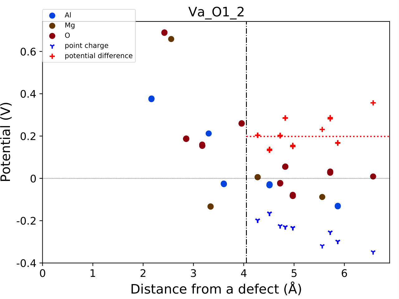
The height of the horizontal line indicates the averaged potential difference between the point-charge potential and the defect-induced potential— specifically, the potential in the defective supercell minus that in the perfect one.
The length of the line indicates the spatial averaging range. For more details, refer to the above publication by Kumagai and Oba (2014).
It is strongly recommended to visually inspect all correction.pdf files
for the calculated defects to avoid mistakes in applying corrections.
11. Check defect structures
We analyze the local structures around defects
using the defect_structure_info (abbreviated as dsi) subcommand:
pydefect dsi -d *_*/
This generates defect_structure_info.json files for each defect directory.
You can view their contents using the pydefect_print command. For example:
 -- defect structure info
Defect type: vacancy
Site symmetry: -3m -> -3m (same)
Has same configuration from initial structure: True
Drift distance: 0.022
Defect center: ( 0.625,  0.375,  0.372)
Removed atoms:
8  Al  ( 0.625,  0.375,  0.375)

Neighbor max distance 2.472
Displacements
Elem  Dist  Displace  Angle  Index  Initial site                  Final site                Neighbor
O     1.9   0.26      160    46     ( 0.639,  0.361,  0.139)  ->  ( 0.647,  0.353,  0.108)  T
O     1.92  0.26      160    42     ( 0.639,  0.139,  0.361)  ->  ( 0.647,  0.110,  0.351)  T
O     1.92  0.26      160    26     ( 0.861,  0.361,  0.361)  ->  ( 0.890,  0.353,  0.351)  T
O     1.92  0.24      170    47     ( 0.389,  0.389,  0.389)  ->  ( 0.360,  0.396,  0.394)  T
O     1.93  0.24      170    31     ( 0.611,  0.611,  0.389)  ->  ( 0.604,  0.639,  0.394)  T
O     1.94  0.23      160    35     ( 0.611,  0.389,  0.611)  ->  ( 0.604,  0.396,  0.637)  T
Al    2.85  0.03      30     14     ( 0.625,  0.125,  0.125)  ->  ( 0.627,  0.128,  0.127)
Al    2.85  0.03      30     21     ( 0.875,  0.375,  0.125)  ->  ( 0.872,  0.373,  0.127)
Al    2.87  0.05      40     16     ( 0.875,  0.125,  0.375)  ->  ( 0.872,  0.128,  0.372)
We can also generate VESTA files to visualize the defect structures
using the defect_vesta_file (abbreviated as dvf) subcommand
in pydefect_util:
pydefect_util dvf -d *_*/
This creates defect.vesta files in each defect directory.
12. Check defect eigenvalues and band-edge states in supercell calculations
Note: This section is optional.
In general, point defects can be classified into three categories:
(1) Defects with deep localized states inside the band gap. These defects are often detrimental to device performance because they can trap carriers. They may also act as color centers, such as vacancies in NaCl. Thus, it is important to identify the location and character of such defect states.
(2) Defects with hydrogenic carrier states, or perturbed host states (PHS). Here, the carriers are weakly bound to the charged defect center near the band edges. Examples include B-on-Si (p-type) and P-on-Si (n-type) substitutional dopants in silicon. These defects are typically not harmful to devices but may introduce carriers or eliminate counter carriers. The wavefunctions of PHS can extend over millions of atoms, so first-principles calculations of their thermodynamic transition levels require very large supercells, which are computationally infeasible. Thus, their charge transition levels are often not calculated directly but assumed to lie near the band edges based on qualitative assessments.
(3) Defects without any states inside the band gap or near the band edges. These defects have little impact on electronic properties as long as their concentrations remain low.
For examples of each case, see our publications:
To distinguish among these types, one must examine the defect energy levels and wavefunctions to determine whether PHS or localized states are present.
pydefect provides tools to analyze eigenvalues and band-edge states as follows:
First, generate perfect_band_edge_state.json
using the perfect_band_edge_state subcommand:
pydefect_vasp pbes -d perfect
Then, generate band_edge_orbital_infos.json files
in the defect directories using the band_edge_orbital_infos subcommand
(abbreviated as beoi):
pydefect_vasp beoi -d *_* -pbes perfect/perfect_band_edge_state.json
This also creates eigenvalues.pdf plots.
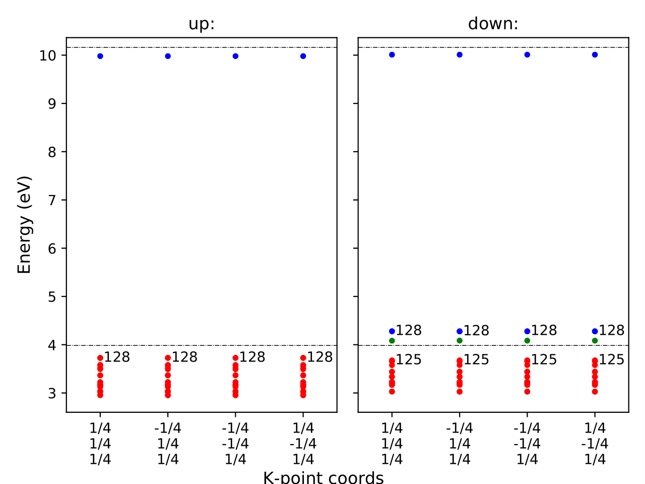
These plots show the single-particle levels and their occupations for spin-up and spin-down channels. The x-axis corresponds to the fractional coordinates of k-points, and the y-axis shows the absolute energy. Each circle represents a state; red, green, and blue denote occupied, partially occupied (0.2–0.8), and unoccupied levels, respectively.
The two horizontal dashed lines indicate the VBM and CBM of the perfect supercell. Band indices are labeled numerically.
Next, generate band_edge_states.json
using the band_edge_states (abbreviated as bes) subcommand:
pydefect bes -d *_*/ -pbes perfect/perfect_band_edge_state.json
To examine this file, use:
pydefect_print band_edge_states.json
Example output:
 -- band-edge states info
Spin-up
     Index  Energy  P-ratio  Occupation  OrbDiff  Orbitals                          K-point coords
VBM  128    3.727   0.33     1.00        0.02     O-p: 0.76                         ( 0.250,  0.250,  0.250)
CBM  129    9.980   0.06     0.00        0.03     Al-s: 0.11, O-s: 0.21, O-p: 0.11  ( 0.250,  0.250,  0.250)
vbm has acceptor phs: False (0.000 vs. 0.2)
cbm has donor phs: False (0.000 vs. 0.2)
---
Localized Orbital(s)
Index  Energy  P-ratio  Occupation  Orbitals

Spin-down
     Index  Energy  P-ratio  Occupation  OrbDiff  Orbitals              K-point coords
VBM  126    4.083   0.67     0.88        0.06     O-p: 0.72             ( 0.250,  0.250,  0.250)
CBM  129    10.010  0.06     0.00        0.01     O-s: 0.21, O-p: 0.11  ( 0.250,  0.250,  0.250)
vbm has acceptor phs: False (0.120 vs. 0.2)
cbm has donor phs: False (0.000 vs. 0.2)
---
Localized Orbital(s)
Index  Energy  P-ratio  Occupation  Orbitals
127    4.277   0.62     0.06        O-p: 2.98
128    4.278   0.62     0.06        O-p: 2.98
The analysis is given for both spin channels.
P-ratio is the participation ratio,
which measures how much of the orbital density is localized
on neighboring atoms (as listed in defect_structure_info.json)
relative to the total over the entire cell.
As mentioned, the formation energies of defects with occupied
donor phs or unoccupied acceptor phs
should typically be excluded from formation energy diagrams.
In pydefect, these classifications are based on the eigenvalues
and the similarity of the wavefunctions to those of the VBM and CBM.
For details, please refer to our upcoming publication.
Note: Automatic classification of PHS and localized states is not always reliable. Users are encouraged to visually inspect the band-edge states and examine band-decomposed charge densities when necessary.
13. Plot defect formation energies
Here, we demonstrate how to plot defect formation energies.
Plotting defect formation energies requires multiple types of information: the band edges, chemical potentials of the competing phases, and the total energies of both perfect and defective supercells.
First, use the defect_energy_infos (= dei) sub-command:
pydefect dei -d *_*/ -pcr perfect/calc_results.json -u ../unitcell/unitcell.yaml -s ../cpd/standard_energies.yaml
This command generates the defect_energy_info.yaml files within each defect directory.
An example is shown below:
name: Va_O1
charge: 0
formation_energy: 6.803585744999999
atom_io:
  O: -1
energy_corrections:
  pc term: 0.0
  alignment term: -0.0
is_shallow: False
Caveats:
(1) The formation_energy is calculated assuming the chemical potentials
of the elements are at their standard states, and the Fermi level is at 0 eV.
(2) Although two energy corrections are included (pc term and alignment term),
you may add custom correction terms if needed.
(3) The is_shallow value will be empty if the previous section (on PHS identification) is skipped.
Here, “shallow” refers to the presence of a perturbed host state (PHS). You may modify
the classification (e.g., shallow/deep) manually if desired.
Next, create the defect_energy_summary.json file using the defect_energy_summary (= des) sub-command:
pydefect des -d *_*/ -u ../unitcell/unitcell.yaml -pbes perfect/perfect_band_edge_state.json -t ../cpd/target_vertices.yaml
This sub-command collects information from each defect_energy_info.yaml
file and compiles it into defect_energy_summary.json.
title: MgAl₂O₄
rel_chem_pots:
 -A Al: 0.00 Mg: -0.69 O: -5.25
 -B Al: 0.00 Mg: -0.32 O: -5.34
 -C Al: -7.87 Mg: -5.94 O: 0.00
 -D Al: -8.01 Mg: -5.66 O: 0.00
vbm: 0.00, cbm: 5.22, supercell vbm: -0.03, supercell_cbm: 6.14

name    atom_io         charge    energy    correction  is_shallow
------  ------------  --------  --------  ------------  ------------
Al_i1   Al: 1               -1    14.958        -0.049  False
                             0     9.896         0.000  True
                             1     3.376         0.527  False
                             2    -0.872         1.814  True
                             3    -6.994         3.370  False
Mg_i1   Mg: 1                0     8.208         0.000  True
                             1     2.015         0.555  True
                             2    -4.117         1.534  False
O_i1    O: 1                -2     8.122         0.721  False
                            -1     7.055         0.149  False
                             0     4.566         0.000  False
Va_Al1  Al: -1              -3    13.527         3.402  False
                            -2    12.968         1.789  True
                            -1    12.672         0.660  True
                             0    12.595         0.000  True
                             1    12.710        -0.232  True
Va_Mg1  Mg: -1              -2    10.093         1.524  False
                            -1     9.580         0.578  True
                             0     9.311         0.000  False
Va_MgO  O: -1 Mg: -1         0     9.887         0.000  False
Va_O1   O: -1                0     6.804         0.000  False
                             1     3.808         0.166  False
                             2     0.883         0.845  False
You can also create a calc_summary.json file using the calc_summary (= cs) sub-command:
pydefect cs -d *_*/ -pcr perfect/calc_results.json
This outputs:
|:---------:|:----------:|:-----------:|:-----------------:|:------------:|:------------------:|:--------------:|
|   name    | Ele. conv. | Ionic conv. | Is energy strange | Same config. |    Defect type     | Symm. Relation |
| Al_i1_-1  |     .      |      .      |         .         |    False     |      unknown       |    subgroup    |
|  Al_i1_0  |     .      |      .      |         .         |    False     |      unknown       |    subgroup    |
|  Al_i1_1  |     .      |      .      |         .         |    False     |      unknown       |    subgroup    |
|  Al_i1_2  |     .      |      .      |         .         |      .       |         .          |       .        |
|  Al_i1_3  |     .      |      .      |         .         |      .       |         .          |       .        |
|  Mg_i1_0  |     .      |      .      |         .         |      .       |         .          |       .        |
|  Mg_i1_1  |     .      |      .      |         .         |      .       |         .          |       .        |
|  Mg_i1_2  |     .      |      .      |         .         |      .       |         .          |       .        |
|  O_i1_-1  |     .      |      .      |         .         |      .       |         .          |       .        |
|  O_i1_-2  |     .      |      .      |         .         |    False     | interstitial_split |    subgroup    |
|  O_i1_0   |     .      |      .      |         .         |      .       |         .          |       .        |
| Va_Al1_-1 |     .      |      .      |         .         |      .       |         .          |       .        |
| Va_Al1_-2 |     .      |      .      |         .         |      .       |         .          |       .        |
| Va_Al1_-3 |     .      |      .      |         .         |      .       |         .          |       .        |
| Va_Al1_0  |     .      |      .      |         .         |      .       |         .          |       .        |
| Va_Al1_1  |     .      |      .      |         .         |      .       |         .          |       .        |
| Va_Mg1_-1 |     .      |      .      |         .         |      .       |         .          |       .        |
| Va_Mg1_-2 |     .      |      .      |         .         |      .       |         .          |       .        |
| Va_Mg1_0  |     .      |      .      |         .         |      .       |         .          |       .        |
| Va_MgO_0  |     .      |      .      |         .         |    False     |      unknown       |      same      |
|  Va_O1_0  |     .      |      .      |         .         |      .       |         .          |       .        |
|  Va_O1_1  |     .      |      .      |         .         |      .       |         .          |       .        |
|  Va_O1_2  |     .      |      .      |         .         |      .       |         .          |       .        |
Note: this feature is still in beta.
Finally, plot the defect formation energies as a function of the Fermi level
using the plot_defect_formation_energy (= pe) sub-command:
pydefect pe -d defect_energy_summary.json -l A
This generates a plot like the following:
To change the chemical potential condition—i.e., select a different vertex from the chemical potential diagram—use the -l option.